Pyspark Code of Machine Learning to Identify Negative Positive Movie Review

How to Predict Sentiment From Picture Reviews Using Deep Learning (Text Classification)

Last Updated on August 27, 2020

Sentiment analysis is a tongue processing problem where text is understood and the underlying intent is predicted.

In this post, you volition observe how you tin predict the sentiment of movie reviews as either positive or negative in Python using the Keras deep learning library.

After reading this post you volition know:

• About the IMDB sentiment assay problem for tongue processing and how to load it in Keras.
• How to utilize word embedding in Keras for natural linguistic communication issues.
• How to develop and evaluate a multi-layer perception model for the IMDB problem.
• How to develop a 1-dimensional convolutional neural network model for the IMDB problem.

Boot-starting time your project with my new book Deep Learning With Python, including step-by-stride tutorials and the Python source code files for all examples.

Let'south get started.

• Update Oct/2016: Updated for Keras 1.i.0 and TensorFlow 0.10.0.
• Update Mar/2017: Updated for Keras 2.0.ii, TensorFlow 1.0.ane and Theano 0.9.0.
• Update Jul/2019: If you are using Keras 2.2.four and NumPy one.16.2+ and go "ValueError: Object arrays cannot exist loaded when allow_pickle=False", then attempt updating NumPy to one.16.1, or update Keras to the version from github, or use the prepare described here.
• Update Sep/2019: Updated for Keras two.2.v.

Predict Sentiment From Movie Reviews Using Deep Learning
Photo by SparkCBC, some rights reserved.

IMDB Motion-picture show Review Sentiment Problem Description

The dataset is the Large Movie Review Dataset often referred to equally the IMDB dataset.

The Large Movie Review Dataset (often referred to every bit the IMDB dataset) contains 25,000 highly polar moving reviews (skilful or bad) for training and the same corporeality again for testing. The problem is to decide whether a given moving review has a positive or negative sentiment.

The data was collected by Stanford researchers and was used in a 2011 paper [PDF] where a split of 50/50 of the information was used for preparation and exam. An accuracy of 88.89% was achieved.

The information was also used as the ground for a Kaggle competition titled "Bag of Words Meets Bags of Popcorn" in late 2014 to early on 2015. Accuracy was achieved to a higher place 97% with winners achieving 99%.

Demand help with Deep Learning in Python?

Take my free 2-week e-mail course and observe MLPs, CNNs and LSTMs (with code).

Click to sign-up now and also get a gratuitous PDF Ebook version of the grade.

Load the IMDB Dataset With Keras

Keras provides access to the IMDB dataset built-in.

The keras.datasets.imdb.load_data() allows yous to load the dataset in a format that is fix for use in neural network and deep learning models.

The words have been replaced by integers that indicate the absolute popularity of the word in the dataset. The sentences in each review are therefore comprised of a sequence of integers.

Calling imdb.load_data() the first fourth dimension will download the IMDB dataset to your estimator and store information technology in your habitation directory nether ~/.keras/datasets/imdb.pkl every bit a 32 megabyte file.

Usefully, the imdb.load_data() provides boosted arguments including the number of top words to load (where words with a lower integer are marked every bit zilch in the returned data), the number of top words to skip (to avoid the "the"'south) and the maximum length of reviews to support.

Let's load the dataset and calculate some properties of it. We volition starting time off past loading some libraries and loading the entire IMDB dataset every bit a preparation dataset.

import numpy from keras . datasets import imdb from matplotlib import pyplot # load the dataset ( X_train , y_train ) , ( X_test , y_test ) = imdb . load_data ( ) X = numpy . concatenate ( ( X_train , X_test ) , axis = 0 ) y = numpy . concatenate ( ( y_train , y_test ) , axis = 0 ) . . .

Next we can display the shape of the training dataset.

. . . # summarize size print ( "Preparation data: " ) print ( X . shape ) impress ( y . shape )

Running this snippet, we can come across that there are l,000 records.

Training data: (50000,) (50000,)

We can besides print the unique class values.

. . . # Summarize number of classes print ( "Classes: " ) impress ( numpy . unique ( y ) )

Nosotros can see that it is a binary classification problem for expert and bad sentiment in the review.

Next we tin can get an idea of the total number of unique words in the dataset.

. . . # Summarize number of words impress ( "Number of words: " ) print ( len ( numpy . unique ( numpy . hstack ( X ) ) ) )

Interestingly, we can see that there are just under 100,000 words across the entire dataset.

Finally, we can become an idea of the boilerplate review length.

. . . # Summarize review length impress ( "Review length: " ) result = [ len ( ten ) for ten in X ] impress ( "Mean %.2f words (%f)" % ( numpy . mean ( upshot ) , numpy . std ( event ) ) ) # plot review length pyplot . boxplot ( result ) pyplot . testify ( )

We can see that the average review has just under 300 words with a standard deviation of just over 200 words.

Review length: Mean 234.76 words (172.911495)

Looking a box and whisker plot for the review lengths in words, we can probably see an exponential distribution that we can probably embrace the mass of the distribution with a clipped length of 400 to 500 words.

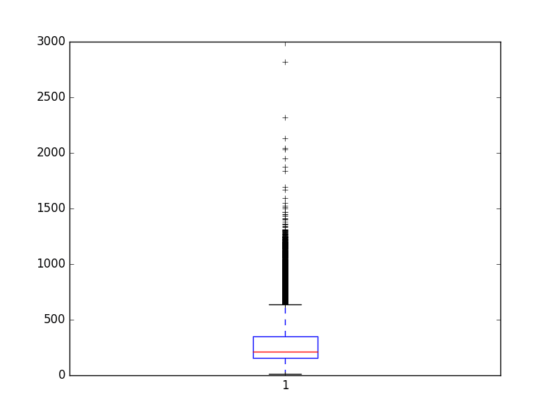
Review Length in Words for IMDB Dataset

Discussion Embeddings

A recent breakthrough in the field of natural language processing is called word embedding.

This is a technique where words are encoded every bit real-valued vectors in a high-dimensional space, where the similarity betwixt words in terms of meaning translates to closeness in the vector space.

Discrete words are mapped to vectors of continuous numbers. This is useful when working with tongue problems with neural networks and deep learning models are we require numbers as input.

Keras provides a convenient manner to catechumen positive integer representations of words into a word embedding past an Embedding layer.

The layer takes arguments that define the mapping including the maximum number of expected words also chosen the vocabulary size (e.g. the largest integer value that will be seen equally an integer). The layer likewise allows you to specify the dimensionality for each discussion vector, called the output dimension.

We would like to use a word embedding representation for the IMDB dataset.

Allow's say that we are only interested in the first v,000 most used words in the dataset. Therefore our vocabulary size will be 5,000. Nosotros can choose to use a 32-dimension vector to represent each word. Finally, nosotros may cull to cap the maximum review length at 500 words, truncating reviews longer than that and padding reviews shorter than that with 0 values.

Nosotros would load the IMDB dataset as follows:

. . . imdb . load_data ( nb_words = 5000 )

Nosotros would and then use the Keras utility to truncate or pad the dataset to a length of 500 for each ascertainment using the sequence.pad_sequences() office.

. . . X_train = sequence . pad_sequences ( X_train , maxlen = 500 ) X_test = sequence . pad_sequences ( X_test , maxlen = 500 )

Finally, later on, the first layer of our model would be an word embedding layer created using the Embedding class as follows:

. . . Embedding ( 5000 , 32 , input_length = 500 )

The output of this beginning layer would be a matrix with the size 32×500 for a given review training or test pattern in integer format.

Now that we know how to load the IMDB dataset in Keras and how to utilise a word embedding representation for it, let'southward develop and evaluate some models.

Elementary Multi-Layer Perceptron Model for the IMDB Dataset

We can start off by developing a simple multi-layer perceptron model with a single hidden layer.

The word embedding representation is a true innovation and we will demonstrate what would have been considered world class results in 2011 with a relatively simple neural network.

Let's first off past importing the classes and functions required for this model and initializing the random number generator to a constant value to ensure nosotros can easily reproduce the results.

# MLP for the IMDB problem from keras . datasets import imdb from keras . models import Sequential from keras . layers import Dumbo from keras . layers import Flatten from keras . layers . embeddings import Embedding from keras . preprocessing import sequence . . .

Next nosotros volition load the IMDB dataset. We will simplify the dataset equally discussed during the department on word embeddings. Only the peak v,000 words will be loaded.

We will also utilise a l%/50% split of the dataset into grooming and examination. This is a good standard separate methodology.

. . . # load the dataset simply only go along the superlative n words, zero the residual top_words = 5000 ( X_train , y_train ) , ( X_test , y_test ) = imdb . load_data ( num_words = top_words )

We will bound reviews at 500 words, truncating longer reviews and nil-padding shorter reviews.

. . . max_words = 500 X_train = sequence . pad_sequences ( X_train , maxlen = max_words ) X_test = sequence . pad_sequences ( X_test , maxlen = max_words )

Now we tin create our model. We volition use an Embedding layer as the input layer, setting the vocabulary to 5,000, the give-and-take vector size to 32 dimensions and the input_length to 500. The output of this first layer volition be a 32×500 sized matrix as discussed in the previous section.

We will flatten the Embedded layers output to one dimension, and so use one dense hidden layer of 250 units with a rectifier activation function. The output layer has one neuron and will use a sigmoid activation to output values of 0 and 1 as predictions.

The model uses logarithmic loss and is optimized using the efficient ADAM optimization procedure.

. . . # create the model model = Sequential ( ) model . add ( Embedding ( top_words , 32 , input_length = max_words ) ) model . add together ( Flatten ( ) ) model . add ( Dumbo ( 250 , activation = 'relu' ) ) model . add ( Dense ( 1 , activation = 'sigmoid' ) ) model . compile ( loss = 'binary_crossentropy' , optimizer = 'adam' , metrics = [ 'accuracy' ] ) print ( model . summary ( ) )

We can fit the model and utilise the examination set as validation while training. This model overfits very quickly so we volition use very few training epochs, in this case simply ii.

In that location is a lot of data so nosotros will use a batch size of 128. Afterward the model is trained, we evaluate its accuracy on the exam dataset.

. . . # Fit the model model . fit ( X_train , y_train , validation_data = ( X_test , y_test ) , epochs = two , batch_size = 128 , verbose = ii ) # Last evaluation of the model scores = model . evaluate ( X_test , y_test , verbose = 0 ) impress ( "Accuracy: %.2f%%" % ( scores [ 1 ] * 100 ) )

Tying all of this together, the complete code list is provided below.

1 2 3 4 5 vi 7 8 ix x eleven 12 13 14 xv 16 17 18 19 twenty 21 22 23 24 25 26

# MLP for the IMDB trouble from keras . datasets import imdb from keras . models import Sequential from keras . layers import Dumbo from keras . layers import Flatten from keras . layers . embeddings import Embedding from keras . preprocessing import sequence # load the dataset merely merely go along the top north words, zero the rest top_words = 5000 ( X_train , y_train ) , ( X_test , y_test ) = imdb . load_data ( num_words = top_words ) max_words = 500 X_train = sequence . pad_sequences ( X_train , maxlen = max_words ) X_test = sequence . pad_sequences ( X_test , maxlen = max_words ) # create the model model = Sequential ( ) model . add ( Embedding ( top_words , 32 , input_length = max_words ) ) model . add together ( Flatten ( ) ) model . add ( Dense ( 250 , activation = 'relu' ) ) model . add ( Dense ( ane , activation = 'sigmoid' ) ) model . compile ( loss = 'binary_crossentropy' , optimizer = 'adam' , metrics = [ 'accurateness' ] ) model . summary ( ) # Fit the model model . fit ( X_train , y_train , validation_data = ( X_test , y_test ) , epochs = 2 , batch_size = 128 , verbose = ii ) # Final evaluation of the model scores = model . evaluate ( X_test , y_test , verbose = 0 ) print ( "Accuracy: %.2f%%" % ( scores [ 1 ] * 100 ) )

Running this example fits the model and summarizes the estimated performance.

Note: Your results may vary given the stochastic nature of the algorithm or evaluation procedure, or differences in numerical precision. Consider running the case a few times and compare the boilerplate outcome.

We tin can run across that this very simple model achieves a score of near 86.94% which is in the neighborhood of the original newspaper, with very piffling effort.

Train on 25000 samples, validate on 25000 samples Epoch 1/2 39s - loss: 0.5160 - acc: 0.7040 - val_loss: 0.2982 - val_acc: 0.8716 Epoch 2/2 37s - loss: 0.1897 - acc: 0.9266 - val_loss: 0.3143 - val_acc: 0.8694 Accuracy: 86.94%

I'chiliad sure we tin do better if we trained this network, perchance using a larger embedding and adding more than hidden layers.

Let'south effort a different network type.

One-Dimensional Convolutional Neural Network Model for the IMDB Dataset

Convolutional neural networks were designed to award the spatial structure in epitome data whilst being robust to the position and orientation of learned objects in the scene.

This same principle can exist used on sequences, such equally the ane-dimensional sequence of words in a motion-picture show review. The same properties that make the CNN model attractive for learning to recognize objects in images can help to larn structure in paragraphs of words, namely the techniques invariance to the specific position of features.

Keras supports 1-dimensional convolutions and pooling past the Conv1D and MaxPooling1D classes respectively.

Again, permit'southward import the classes and functions needed for this example and initialize our random number generator to a constant value so that we tin can easily reproduce results.

# CNN for the IMDB problem from keras . datasets import imdb from keras . models import Sequential from keras . layers import Dense from keras . layers import Flatten from keras . layers . convolutional import Conv1D from keras . layers . convolutional import MaxPooling1D from keras . layers . embeddings import Embedding from keras . preprocessing import sequence

Nosotros can as well load and prepare our IMDB dataset every bit we did before.

. . . # load the dataset but but proceed the peak n words, zip the rest top_words = 5000 ( X_train , y_train ) , ( X_test , y_test ) = imdb . load_data ( num_words = top_words ) # pad dataset to a maximum review length in words max_words = 500 X_train = sequence . pad_sequences ( X_train , maxlen = max_words ) X_test = sequence . pad_sequences ( X_test , maxlen = max_words )

Nosotros can now ascertain our convolutional neural network model. This time, after the Embedding input layer, we insert a Conv1D layer. This convolutional layer has 32 feature maps and reads embedded discussion representations 3 vector elements of the word embedding at a time.

The convolutional layer is followed by a 1D max pooling layer with a length and stride of 2 that halves the size of the feature maps from the convolutional layer. The rest of the network is the same every bit the neural network above.

. . . # create the model model = Sequential ( ) model . add ( Embedding ( top_words , 32 , input_length = max_words ) ) model . add ( Conv1D ( filters = 32 , kernel_size = 3 , padding = 'aforementioned' , activation = 'relu' ) ) model . add ( MaxPooling1D ( pool_size = 2 ) ) model . add together ( Flatten ( ) ) model . add ( Dense ( 250 , activation = 'relu' ) ) model . add ( Dumbo ( i , activation = 'sigmoid' ) ) model . compile ( loss = 'binary_crossentropy' , optimizer = 'adam' , metrics = [ 'accuracy' ] ) model . summary ( )

We also fit the network the same every bit before.

. . . # Fit the model model . fit ( X_train , y_train , validation_data = ( X_test , y_test ) , epochs = 2 , batch_size = 128 , verbose = 2 ) # Final evaluation of the model scores = model . evaluate ( X_test , y_test , verbose = 0 ) print ( "Accurateness: %.2f%%" % ( scores [ one ] * 100 ) )

Tying all of this together, the complete code listing is provided below.

1 2 3 4 5 6 7 8 9 10 11 12 thirteen fourteen 15 sixteen 17 18 19 20 21 22 23 24 25 26 27 28 29 thirty 31

# CNN for the IMDB problem from keras . datasets import imdb from keras . models import Sequential from keras . layers import Dumbo from keras . layers import Flatten from keras . layers . convolutional import Conv1D from keras . layers . convolutional import MaxPooling1D from keras . layers . embeddings import Embedding from keras . preprocessing import sequence # load the dataset but simply keep the height n words, zero the rest top_words = 5000 ( X_train , y_train ) , ( X_test , y_test ) = imdb . load_data ( num_words = top_words ) # pad dataset to a maximum review length in words max_words = 500 X_train = sequence . pad_sequences ( X_train , maxlen = max_words ) X_test = sequence . pad_sequences ( X_test , maxlen = max_words ) # create the model model = Sequential ( ) model . add together ( Embedding ( top_words , 32 , input_length = max_words ) ) model . add ( Conv1D ( 32 , iii , padding = 'same' , activation = 'relu' ) ) model . add ( MaxPooling1D ( ) ) model . add ( Flatten ( ) ) model . add ( Dense ( 250 , activation = 'relu' ) ) model . add together ( Dumbo ( ane , activation = 'sigmoid' ) ) model . compile ( loss = 'binary_crossentropy' , optimizer = 'adam' , metrics = [ 'accuracy' ] ) model . summary ( ) # Fit the model model . fit ( X_train , y_train , validation_data = ( X_test , y_test ) , epochs = 2 , batch_size = 128 , verbose = 2 ) # Concluding evaluation of the model scores = model . evaluate ( X_test , y_test , verbose = 0 ) print ( "Accuracy: %.2f%%" % ( scores [ 1 ] * 100 ) )

Running the case, we are showtime presented with a summary of the network construction. We tin can run into our convolutional layer preserves the dimensionality of our Embedding input layer of 32-dimensional input with a maximum of 500 words. The pooling layer compresses this representation by halving it.

Annotation: Your results may vary given the stochastic nature of the algorithm or evaluation procedure, or differences in numerical precision. Consider running the example a few times and compare the average outcome.

Running the example offers a modest but welcome comeback over the neural network model above with an accuracy of nearly 87.79%.

Train on 25000 samples, validate on 25000 samples Epoch i/2 38s - loss: 0.4451 - acc: 0.7640 - val_loss: 0.3107 - val_acc: 0.8660 Epoch two/ii 39s - loss: 0.2373 - acc: 0.9064 - val_loss: 0.2909 - val_acc: 0.8779 Accuracy: 87.79%

Over again, there is a lot of opportunity for further optimization, such as the use of deeper and/or larger convolutional layers.

One interesting idea is to set up the max pooling layer to use an input length of 500. This would compress each characteristic map to a single 32 length vector and may boost performance.

Summary

In this post, you discovered the IMDB sentiment analysis dataset for natural language processing.

You learned how to develop deep learning models for sentiment assay including:

• How to load and review the IMDB dataset within Keras.
• How to develop a large neural network model for sentiment analysis.
• How to develop a one-dimensional convolutional neural network model for sentiment analysis.

Do you have any questions near sentiment analysis or this mail? Ask your questions in the comments and I volition do my best to respond.

Develop Deep Learning Projects with Python!

 What If You Could Develop A Network in Minutes

...with just a few lines of Python

Detect how in my new Ebook:
Deep Learning With Python

It covers cease-to-terminate projects on topics like:
Multilayer Perceptrons,Convolutional Nets andRecurrent Neural Nets, and more than...

Finally Bring Deep Learning To
Your Own Projects

Skip the Academics. Just Results.

Run into What's Inside

lindseyquiters.blogspot.com

Source: https://machinelearningmastery.com/predict-sentiment-movie-reviews-using-deep-learning/

Share this post